The Inverse CDF Method
Hello. This post is a math and probability post. I will talk about generating non-uniform random variables/numbers with the Inverse CDF Method. The inverse CDF method involves computing quantiles from probabilities and using standard uniform random variables to generate non-uniform random variables.
This topic relates to Probability Theory, and Monte Carlo Simulations.
Table of Contents
- Introduction
- The Uniform Random Variable
- The Cumulative Distribution Function (CDF)
- The Inverse CDF Method For Generating Non-Uniform Random Numbers
- Examples of the Inverse CDF Method
Introduction
Generating random numbers allows us to simulate natural random events without the actual events occurring. For example, instead of flipping a coin 1000 times, we can use software to simulate or emulate this for us.
There is a lot of utility and usefulness in generating random numbers (and/or variables). Applications include finding averages, estimating the mean or frequency/probability distribution, extracting data for decision making and so on.
The Uniform Random Variable
The uniform random variable is a continuous random variable which takes on values from parameters \(a\) to \(b\). If \(V\) is a uniform random variable the we denote the random variable \(V\) as \(V \sim \text{Unif}(a,b)\). The uniform random variable takes on any value between a and b, inclusive.
The continuous probability distribution of a uniform random variable is:
\[\displaystyle f(v) = \dfrac{1}{b - a}\]
If the parameters \(a\) and \(b\) are 0 and 1 respectively then \(V\) is a standard uniform random variable \(U\). It would be denoted as \(U \sim \text{Unif}(0,1)\). The continuous probability distribution of a standard uniform random variable is just \(f(u) = \dfrac{1}{1 - 0} = 1\).
The Cumulative Distribution Function (CDF)
The Cumulative Distribution Function or the CDF is the probability that a real-valued random variable \(X\) with a given probability distribution is less than or equal to a quantity \(x\). It is often denoted by \(F(x) = P(X \leq x)\).
Some CDF Properties
The CDF is a non-decreasing function.
\(\displaystyle \lim_{x\rightarrow\infty} F(x) = 1\) (An upper bound and horizontal asymptote at \(F(x) = 1\) if \(x\) approaches \(\infty\).)
\(\displaystyle \lim_{x\rightarrow -\infty} F(x) = 0\) (A lower bound and horizontal asymptote at \(F(x) = 0\) if \(x\) approaches -infinity.)
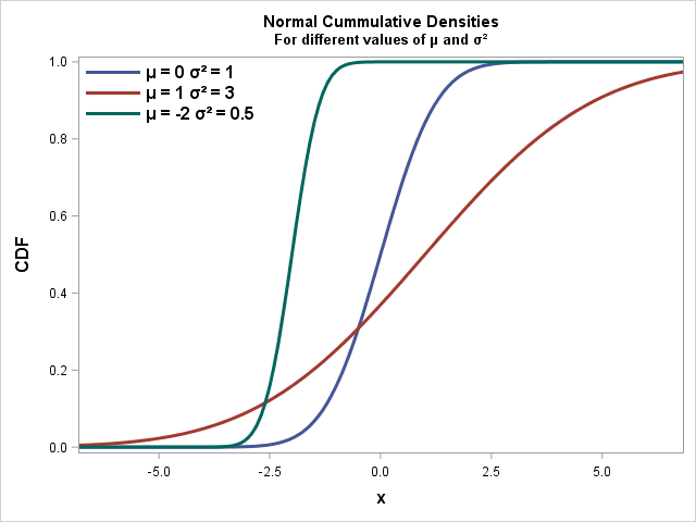
The following image of a sample CDF summarizes the above three properties. This image is for a standard normal distribution.
For a uniform random variable, the CDF is \(X \sim \text{Unif}(a,b)\) is \(F(x) = \dfrac{x - a}{b - a}\).
Proof
\[\displaystyle F(x) = P(X \leq x) = \int_{a}^{x} \dfrac{1}{b-a} = \dfrac{x - a}{b - a}\]
For the case of a standard uniform random variable, substituting \(b = 1\) and \(a = 0\) yields the CDF as \(F(x) = x\).
The Inverse CDF Method For Generating Non-Uniform Random Numbers
We have discovered that the standard uniform random variable takes on values between 0 and 1 inclusive. The CDF of a (continuous) distribution also takes on values between 0 and 1 inclusive. In addition, the inverse CDF \(F^{-1}(x)\) is also an increasing function (of \(x\)). These facts are used when using the Inverse CDF Method for generating non-uniform random numbers.
We now have the necessary background to understand the Inverse CDF Method. We use uniform random variables to generate non-uniform random variables. The algorithm is as follows:
Obtain or generate a draw (realization) \(u\) from the standard uniform distribution \(U \sim \text{Unif}(0,1)\)
The draw \(x\) from the CDF \(F(x)\) is given by \(x = F^{-1}(u)\).
Examples of the Inverse CDF Method
Example One
Suppose we only know how to generate or sample Unif(0,1) random variables. We want to generate Unif(a,b) random variables. The Inverse CDF Method allows us to do this as follows.
The CDF of Unif(a,b) is \(F(x) = \dfrac{x - a}{b - a}\) for any \(x\) in the open interval \((a, b)\). To obtain the inverse CDF, we solve for \(x\) in \(F(x) = u = \dfrac{x - a}{b - a}\).
The resulting inverse CDF is \(F^{-1}(u) = a + (b - a)u\).
To generate a Unif(a, b) random variable \(X\) from a random variable \(U \sim \text{Unif}0,1)\), we would set the random variable X as:
\[\displaystyle X = a + (b-a)U\]
A check can be made for a = 0 and b = 1 to see that \(X = U \sim \text{Unif}(0,1)\).
Example Two
In this example, we generate an exponential random variable with \(x > 0\) and the rate lambda as \(\lambda > 0\). The continuous probability distribution of the exponential random variable is:
\[\displaystyle f(x) = \lambda \text{e}^{-\lambda x}\]
Integrating \(f(x)\) with bounds from 0 to x gives:
\[\displaystyle F(x) = \int_{0}^{x} \lambda \text{e}^{-\lambda u} \text{ du} = 1 - \text{e}^{-\lambda x}\].
Solving for \(x = F^{-1}(u)\) in \(1 - \text{e}^{-\lambda x}\) gives us \(x = -\dfrac{1}{\lambda} ln(1 - u)\).
The formula for X is \(X = -\dfrac{1}{\lambda} \text{ln}(1 - U)\). Alternatively, we can use \(X = -\dfrac{\text{ln}(U)}{\lambda}\) since \((1 - U) \sim \text{Unif}(0, 1)\) from \(U \sim \text{Unif}(0,1)\).
Example Three
This third example deals with the Pareto distribution. Given the shape parameter \(k\) and the scale parameter \(\lambda\), the Pareto distribution has a probability density function (pdf) of:
\[f(x) = \dfrac{k \lambda^k}{x^{(k + 1)}} \text{ for } x > \lambda\]
The cumulative distribution function (CDF) of the Pareto distribution involved integrating with bounds from \(\lambda\) to \(x\).
\[F(x) = P(X \leq x) = \int_{\lambda}^{x} \dfrac{k \lambda^k}{t^{(k + 1)}} \text{ dt } \]
\[F(x) = \dfrac{k \lambda^k t^{-k}}{-k} \Bigg|_{t = \lambda}^{t = x} \]
\[F(x) = \dfrac{k \lambda^k x^{-k}}{-k} - \dfrac{k \lambda^k \lambda^{-k}}{-k} \]
\[F(x) = - \lambda^k x^{-k} + 1 \]
\[F(x) = 1 - (\dfrac{\lambda}{x})^{k} \]
To find the generating formula, set \(F(x) = u\) and solve for \(x = F^{-1}(u)\). This u could be replaced by the standard uniform random variable \(U\).
\[u = 1 - (\dfrac{\lambda}{x})^{k}\]
\[ u - 1 = - (\dfrac{\lambda}{x})^{k}\]
\[ 1 - u = (\dfrac{\lambda}{x})^{k}\]
\[ x^k = \dfrac{\lambda^k}{1 - u}\]
\[x = F^{-1}(u) = \frac{\lambda}{(1 - u)^{1/k}}\]
The generating formula would be \(F^{-1}(U) = \frac{\lambda}{(1 - U)^{1/k}}\) with \(U \sim \text{Unif}(0,1)\). You could replace \((1 - U)\) with just \(U\) since both \((1 - U)\) and \(U\) are standard uniform random variables.
References
- Financial Mathematics: A Comprehensive Treatment by Giuseppe Campolieti and Roman N. Makarov
- http://www.math.wm.edu/~leemis/chart/UDR/PDFs/Pareto.pdf
- http://isites.harvard.edu/fs/docs/icb.topic1475777.files/stat110hw5solutions.pdf