Brownian Motion
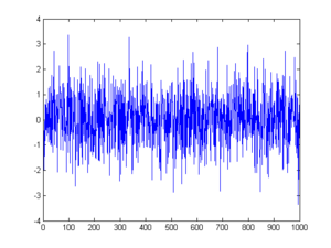
The image is from http://experimentationlab.berkeley.edu/node/83.
Hello. This post will be about Brownian Motion. This topic is a probability and stochastic calculus topic.
Prerequisites and Audience
This topic appeals to the probability and financial mathematics audience. One should be familiar with the normal distribution. It would also be helpful to read another previous article on the random walk.
What Is Brownian Motion?
Brownian Motion is a stochastic (random) process which is a normal distribution with a mean of 0 and a variance of time t. The variance of Brownian motion varies over time.
Brownian Motion is a normal random variable and is denoted by \(W_{t} \sim N(0, t)\). Sometimes \(B_{t}\) is used instead of \(W_{t}\) and sometimes you see \(W(t)\) or \(B(t)\) instead of \(W_{t}\) or \(B_{t}\).
From Random Walks to Brownian Motion
The derivation of Brownian Motion comes from the random walk. In fact, it comes from the scaled symmetric random walk. The scaled symmetric random walk is defined by:
\[\displaystyle W^{(n)}(t) = \dfrac{1}{\sqrt{n}}M_{nt}\]
with \(M_{nt} = \displaystyle\sum_{j=1}^{nt} X_j\), \(nt\) being a positive integer and:
\[ X_j = \begin{cases} +1, & \text{if }\omega_j = \text{Heads } \\ -1, & \text{if }\omega_j =\text{Tails}\end{cases}\]
Central Limit Theorem
Letting \(t \geq 0\) be fixed. As n approaches infinity, then at time t the distribution of the scaled random walk $ W^{(n)}(t)$ converges to a normal distribution with mean 0 and variance t.
The limit of these scaled random walks \(W^{(n)}(t)\) as \(n \rightarrow \infty\) is Brownian motion.
Properties
Some basic properties of Brownian Motion include:
\[W(0) = W_{0} = 0\]
\[E[W_{t}] = 0\]
\[Var[W_{t}] = t\]
Covariance of Brownian Motion
If we have two times \(s\) and \(t\) with \(s < t\) the covariance of \(W_{s}\) and \(W_{t}\) is the minimum of the times \(s\) and \(t\) which is time \(s\). In notation, we have:
\[ \displaystyle \text{Cov}(W(s), W(t)) = E[\,(W_{s} - E[W_{s}] \,)\, (W_{t} - E[W_{t}]) \,] \, = E[W_{s} W_{t}] = s .\]
The Moment Generating Function of Brownian Motion
The moment generating function (mgf) of a normal random variable X is given by
\[M_{X}(s) = E[\text{e}^{sX}] = \text{e}^{\mu s + \sigma^2 s^2 / 2}\].
Since Brownian Motion is \(W_{t} \sim N(0, t)\), the moment generating function of Brownian motion would be
\[E[\text{e}^{sW_{t}}] = E[\text{e}^{t s^2/2}]\].
Martingale Property of BM
Brownian Motion is a martingale. In mathematical notation that is:
\[E[W_{t} | \mathcal{F}_{s}] = W_{s}\]
with times \(s\) and \(t\) and \(s < t\).
This means that the expectation of Brownian motion at time t given the filtration or history of the random process up to time s is just Brownian Motion at time s. For example, the expectation of Brownian motion at a later time given the present time is just Brownian motion at the present.
Independent Brownian Increments
For \(0 = t_{0} < t_{1} < ... < t_{m}\), the increments:
\[\displaystyle W_{t_{1}} - 0 = W_{t_{1}} - W_{t_{0}} \, , \, W_{t_{2}} - W_{t_{1}} \, , \, ... , W_{t_{m}} - W_{t_{m - 1}}\]
are independent of each other and their means are zero.
Their variances are
\[\text{Var}(W_{t_{m}} - W_{t_{m - 1}}) = t_{m} - t_{m-1}\].
Covariance-Variance Matrix of Brownian Motion
Since each Brownian increment from above are independent and normally distributed, the random variables \(W(t_{1}), ... , W(t_{m})\) are jointly normally distributed.
The mean vector of the \(m\)-dimensional vector \((W(t_{1}), W(t_{2}), ... , W(t_{m}))\) is the zero vector.
From before we had the covariance of Brownian Motion as \(s\) assuming that \(s\). In the covariance-variance matrix for Brownian motion, each \((i, j)\) entry is \(\text{Cov}(W_{i}, W_{j}) = \text{min}(i ,j)\)
For example if we have the first row and second column entry in the covariance matrix, we have \(\text{Cov}(W_{1}, W_{2}) = 1\) as \(i =1 < j = 2\).
Assume that we have the ordered times \(0 = t_{0} < t_{1} < ... < t_{m}\). The m by m covariance-variance matrix of the \(m\)-dimensional vector \((W(t_{1}), W(t_{2}), ... , W(t_{m}))\) is as follows:
\[\begin{bmatrix} \text{Cov}(W_{1}, W_{1}) & \text{Cov}(W_{1}, W_{2}) & \dots & \text{Cov}(W_{1}, W_{m}) \\ \text{Cov}(W_{2}, W_{1}) & \text{Cov}(W_{2}, W_{2}) & \dots & \text{Cov}(W_{2}, W_{m}) \\ \vdots & \vdots & \ddots & \vdots \\ \text{Cov}(W_{m}, W_{1}) & \text{Cov}(W_{m}, W_{2}) & \dots & \text{Cov}(W_{m}, W_{m}) \\ \end{bmatrix} = \begin{bmatrix} t_{1} & t_{1} & \dots & t_{1} \\ t_{1} & t_{2} & \dots & t_{2} \\ \vdots & \vdots & \ddots & \vdots \\ t_{1} & t_{2} & \dots & t_{m}\\ \end{bmatrix}\]
Note that for \(i = 1, 2, 3, ... , m, \text{Cov}(W_{i}, W_{i}) = \text{Var}(W_{i}, W_{i}) = t_{i}\).
Notes
The covariance-variance matrix and covariance matrix refer to the same matrix.
Topics such as filtration and the Brownian Motion reflection principle are not discussed in depth for simplicity.
Multidimensional Brownian Motion is a more difficult case. Here we are mostly in one dimension.
Brownian Motion is sometimes called the Wiener process. Don’t ask me why.
Reference
Certain parts of this material was taken from the book Stochastic Calculus for Finance II - Continuous Time Models by Steven E. Shreve.